A 3D tour over Lake Geneva with rayshader
If you follow the #rstats news on Twitter, you have most likely seen the impressive 3D maps produced with Tyler Morgan-Wall’s rayshader package. I’ve been wanting to try it for a long time and I finally found the time to do it last week. As a limnologist living on the shores of Lake Geneva, I didn’t hesitate for long about the location of my first map, which, in the excitement of the moment, I immediately published on twitter.
Finally I found time to dive into @tylermorganwall rayshader #rstats 📦! To start, here is a 3D rendering of Lake Geneva and my workplace @UmrCarrtel. Stay tuned, there's a blog post and more exciting stuffs to come! pic.twitter.com/3VpPcYIdO8
— Francois Keck (@FrancoisKeck) September 26, 2019
In this tweet I was promising to go deeper into the subject. That’s the purpose of this post.
First, we load some packages, functions and data. I have prepared a geotiff file for the region of interest (the surroundings of Lake Geneva). The elevation data were extracted from the SRTM 30 m dataset (thanks @tylermorganwall for the advice!) and I have completed the DEM with a low-resolution model of the lake bathymetry. There is a very high-resolution bathymetry available for lake Geneva, but sadly not released in open data. Finally, we will also need a simple shapefile of the lake shoreline.
library(raster)
library(magrittr)
library(stringr)
library(rgl)
library(rayshader)
library(magick)
library(ggplot2)

source("https://gist.github.com/fkeck/4820db83b9ff2fbf1f7fe901563ddc82/raw/")

# Some useful functions by Will Bishop from his post on rayshader
# https://wcmbishop.github.io/rayshader-demo/
source("https://raw.github.com/wcmbishop/rayshader-demo/master/R/rayshader-gif.R")

mnt <- raster("combined_leman.tif")
mnt <- aggregate(mnt, 2) # Simplification factor

ccv <- rgdal::readOGR("ccv.shp")

plot(mnt)
plot(ccv, add = T)

export_folder <- "/home/francois/Documents/rayshader"

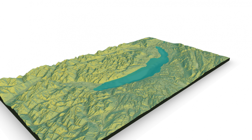
Now, we are ready to render our first 3D scene! The rayshader API makes the task extremely easy. Starting from the elevation matrix, we successively add shadow layers and print the result on screen with OpenGL.
#### Static rendering ####
elmat <-  matrix(raster::extract(mnt, raster::extent(mnt), buffer = 1000),
                 nrow = ncol(mnt), ncol = nrow(mnt))
z_scale <- 40

ambmat <- ambient_shade(elmat)
raysha <- ray_shade(elmat, zscale = z_scale, maxsearch = 300)
hillshade <- elmat %>%
  sphere_shade(texture = "imhof1", sunangle = 35) %>%
  add_shadow(raysha, 0.5) %>%
  add_shadow(ambmat, 0.5)

plot_3d(hillshade, elmat, zscale = z_scale, windowsize = c(1400, 620))
render_camera(theta = 135, phi = 25, zoom = 0.4, fov = 75)
render_water(elmat, zscale = z_scale, wateralpha = 0.7,
             watercolor = "turquoise4", waterdepth = 372,
             waterlinecolor = "lightblue", waterlinealpha = 0.5)
render_snapshot(file.path(export_folder, "static_leman.png"))

Ok, now that we have 3D, what about adding a 4th dimension with time? I have to admit that it was the animations made with rayshader that impressed me the most in the first place. The coolest thing was probably this video of Monterey Bay showing water level progressively increasing and decreasing in an infinite, hypnotizing loop. I definitely needed to have the same thing done with the lake I see every day by my window.
#### Water filling animation ####
list.files(export_folder, pattern = "render_", full.names = TRUE) %>%
  file.remove()

n_frames <- 300
thetas <- transition_values(from = -45, to = -225, steps = n_frames)
water_level <- transition_values(from = 372, to = 0, steps = n_frames)

plot_3d(hillshade, elmat, zscale = z_scale, windowsize = c(1400, 620))

for(i in 1:n_frames){

  file_img_i <- file.path(export_folder, paste0("render_", sprintf("%04d", i), ".png"))

  render_camera(theta = thetas[i], phi = 25, zoom = 0.4, fov = 75)
  render_water(elmat, zscale = z_scale, wateralpha = 0.7,
               watercolor = "turquoise4", waterdepth = water_level[i])

  render_snapshot(file_img_i)
}

paste0('cd ', export_folder, '  && ffmpeg -y -r 25 -i render_%04d.png',
       ' -c:v libx264 -vf "fps=25,format=yuv420p" filling_movie.mp4') %>%
  system()
The camera movement reinforces the 3D perception but I am a little disappointed by the “filling” of the lake. The low resolution of the bathymetry gives a poor result here.
So far, I have simply adapted bits of code found here and there. Now, it is time to try something a bit more exciting. For that I will need new data. My colleague and friend Frédéric Soulignac has developed a 3D hydrodynamic model for the lake temperature and he is kind enough to share some of his simulation outputs for my little experiments. My idea is to project the simulated surface temperatures onto the lake surface. Fred provided several days of data, so I have the opportunity to make a nice animation.
Technically, I use a height-field surface shape added to the 3D scene with the rgl.surface function. The surface is flat, the height is fixed at the altitude of the lake (372m), locations are colored according to the temperature data and the height of the points outside the lake is set to NA, so that they are not drawn. It is also important to set the lit argument on FALSE to disable the calculation of light effects on this object. To complete the graph, we will add some elements: the date and time, a color scale bar and a temperature histogram. I didn’t try to integrate these elements directly into the 3D scene. Instead, I added them after the rendering, using the magic drawing functions of the magick package.
#### Temperature animation ####

# Load the temperature data. These are raster objects imported from Matlab.
# We need to adjust projection and resolution to fit with mnt
load("/home/francois/Documents/fred_temp.RData")

temp_interp_crop <- lapply(temp_interp_list, function(x) {
  projectRaster(x, mnt) %>% extend(mnt)
})

# We prepare the color palette
all_temps <- do.call(rbind, temp_list)$temperature
pal <- viridisLite::viridis(100)
pal <- viridisLite::inferno(100)
pal_cut <- seq(min(all_temps), max(all_temps), by = (max(all_temps) - min(all_temps))/100)
names(pal) <- levels(cut(all_temps, pal_cut))

# Color matrix for the surface
colmat_list <- lapply(temp_interp_crop, function(temp_interp_crop){
  colmat <- matrix(raster::extract(temp_interp_crop, raster::extent(temp_interp_crop), buffer = 1000),
                   ncol = nrow(temp_interp_crop), nrow = ncol(temp_interp_crop))
  colmat <- matrix(pal[cut(colmat, pal_cut)], nrow = nrow(colmat), ncol = ncol(colmat))
  return(colmat)
})

# Color height for the surface
z_height <- matrix(372, nrow = nrow(colmat_list[[1]]), ncol = ncol(colmat_list[[1]]))
z_height[which(is.na(colmat_list[[1]]))] <- NA

n_frames <- 500
thetas <- transition_values(from = -45, to = -225, steps = n_frames)
zoom <- transition_values(from = 0.6, to = 0.3, steps = n_frames)
temp_idx <- transition_values(from = 1, to = length(colmat_list),
                              steps = n_frames, type = "lin", one_way = TRUE) %>% round(0)

# We load a color scale bar picture in memory
img_scale <- image_graph(width = 195, height = 50)
par(mar = c(3, 0, 0, 0))
col_bar_h(pal, min(all_temps), max(all_temps), n.tick = 2)
dev.off()


plot_3d(hillshade, elmat, zscale = z_scale, windowsize = c(1400, 620))

list.files(export_folder, pattern = "render_", full.names = TRUE) %>%
  file.remove()

for(i in seq_len(n_frames)){

  file_img_i <- file.path(export_folder, paste0("render_", sprintf("%04d", i), ".png"))

  render_camera(theta = thetas[i], phi = 25, zoom = zoom[i], fov = 75)
  rgl.surface((1:nrow(colmat_list[[temp_idx[i]]])),
              (1:ncol(colmat_list[[temp_idx[i]]])) - ncol(colmat_list[[temp_idx[i]]]),
              z_height/z_scale,
              color = colmat_list[[temp_idx[i]]], back = "lines", lit = FALSE)
  render_snapshot2(file_img_i)
  rgl.pop()

  img_histo <- image_graph(width = 300*0.8, height = 150*0.8)
    print(
      temp_list[[temp_idx[i]]] %>%
      ggplot() +
      geom_histogram(aes(temperature, fill = cut(temperature, pal_cut)), bins = 30) +
      geom_hline(yintercept = 0, size = 0.7) +
      scale_color_manual(values = pal) +
      scale_fill_manual(values = pal) +
      theme_void() +
      theme(legend.position = "none") +
      xlim(16, 24)
    )
  dev.off()

  img <- image_read(file_img_i)

  img <- image_composite(img, img_scale, offset = "+1160+50")
  img <- image_composite(img, img_histo, offset = "+20+10")

  img <- image_draw(img, xlim = c(0, image_info(img)[["width"]]), ylim = c(0, image_info(img)[["height"]]))
  text(1260, 580, expression(paste("Temperature (", degree, "C)")), cex = 1.2)
  text(625, 565, str_split(temp_date_list[[temp_idx[i]]], " ", simplify = TRUE)[1], cex = 2, adj = 0.5)
  text(775, 565, str_split(temp_date_list[[temp_idx[i]]], " ", simplify = TRUE)[2], cex = 2, adj = 0.5)
  dev.off()
  image_write(img, path = file_img_i)
  print(i)
}


paste0('cd ', export_folder, '  && ffmpeg -y -r 25 -i render_%04d.png',
       ' -c:v libx264 -vf "fps=25,format=yuv420p" temp_movie2.mp4') %>%
  system()
HD version
Okay, that’s all for now. I am very satisfied with the result. And so is Fred 🙂 There are so many other things to do with rayshader but it will be for later.